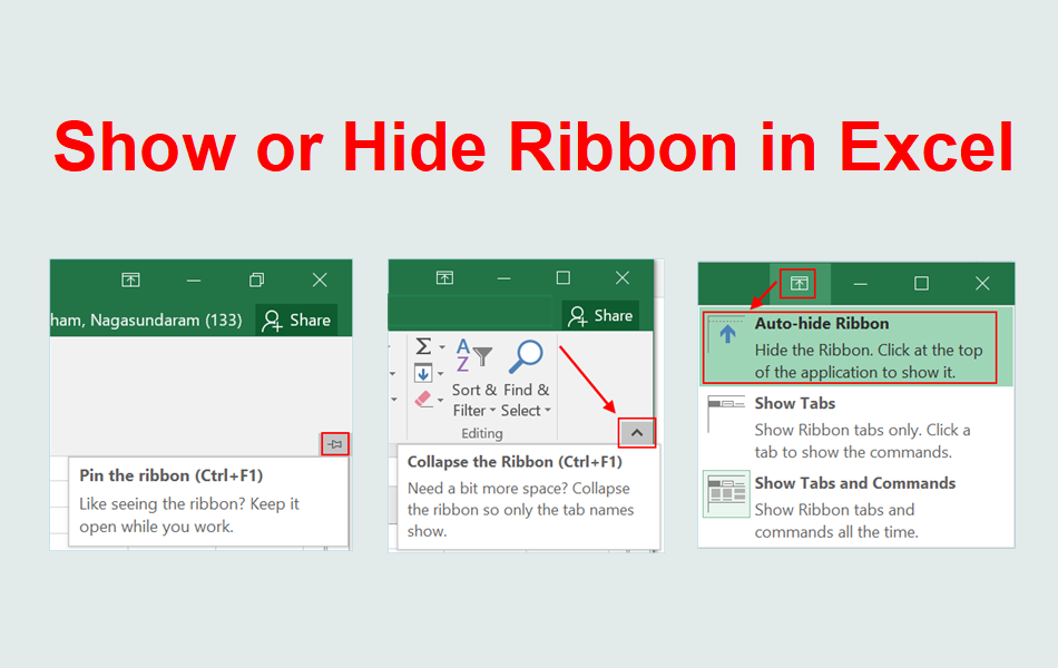
How to show or hide the Excel ribbon in Windows and Mac

The content area in an Excel workbook is usually small. The ribbon area occupies the top of Excel and contains tool icons and text descriptions for each menu tab. When you have a larger Excel worksheet, you should get rid of the ribbon area to get a convenient space. It also makes sense to show or hide the ribbon when needed. In this article, let’s discuss how to show or hide the ribbon in Excel on Windows and MacBook.

Although we have explained it using Excel, all these tips apply to all Microsoft Office applications like Excel, Word, and PowerPoint.

Show or Hide the Ribbon in Windows

1. Use the Arrow Buttons

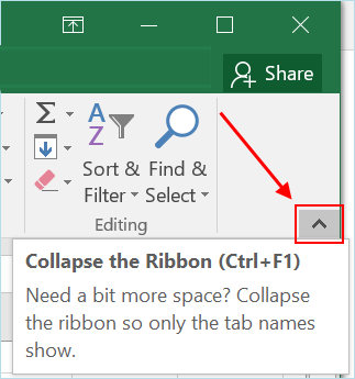
The easiest way is to click the small upward arrow that appears at the right end of the ribbon. This will hide the ribbon that displays all menu items, giving the cells some visible area.

2. Right-click and hide the Ribbon

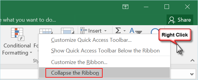
Simply right-click anywhere in the Ribbon area and select the “Collapse Ribbon” option. This will perform the same function as the arrow button and hide the ribbon.

3. Use shortcut keys

Okay, you’ve got a problem with that little arrow. After you hide the ribbon, the arrow disappears, too, because it’s part of the ribbon, too. Now you need to break your head to enable the ribbon again, because you need those menu options. The same problem exists with right-clicking and collapsing the ribbon.

This is a handy shortcut. Simply press the “Ctrl + F1” keys to open or close the ribbon. This means you can hide and show the ribbon by pressing these shortcuts. We recommend using this shortcut instead of using arrows or right-clicking to hide the ribbon. This should also work for Word, PowerPoint, and all Microsoft applications.

4. Auto-Hide Ribbon

You can also automatically hide the ribbon and show it only when you click on the top bar. Click the arrow button that appears next to it to minimize the icon. Select the “Auto-Hide Ribbon” option.

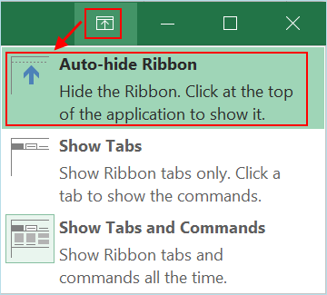
Now the ribbon will disappear and you will be using excel like in full screen mode. If you want to enable the ribbon again, click on the three dots in the top bar, which will temporarily show the ribbon.

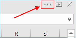
To enable it permanently, click on the arrow button again and select the “Show Tabs” or “Show Tabs and Commands” option.

5. Pin the Ribbon

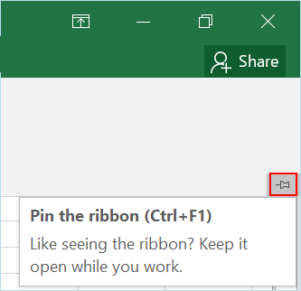
The last option is to pin your Ribbon. Follow these steps to pin the Ribbon on Excel:

• First press “Control + F1” to hide the Ribbon.
• Click on any menu item to see the Ribbon again.
• Now you will see a small pushpin icon on the bottom right corner of the Ribbon.
• Click on it and pin the Ribbon. This will ensure that the Ribbon is always there when you are working on that spreadsheet.

Customize the Ribbon in Windows

Right-click on the Ribbon area and select the Customize Ribbon option. You will see the Excel Options pop-up window displaying the options in the Customize the Ribbon section.

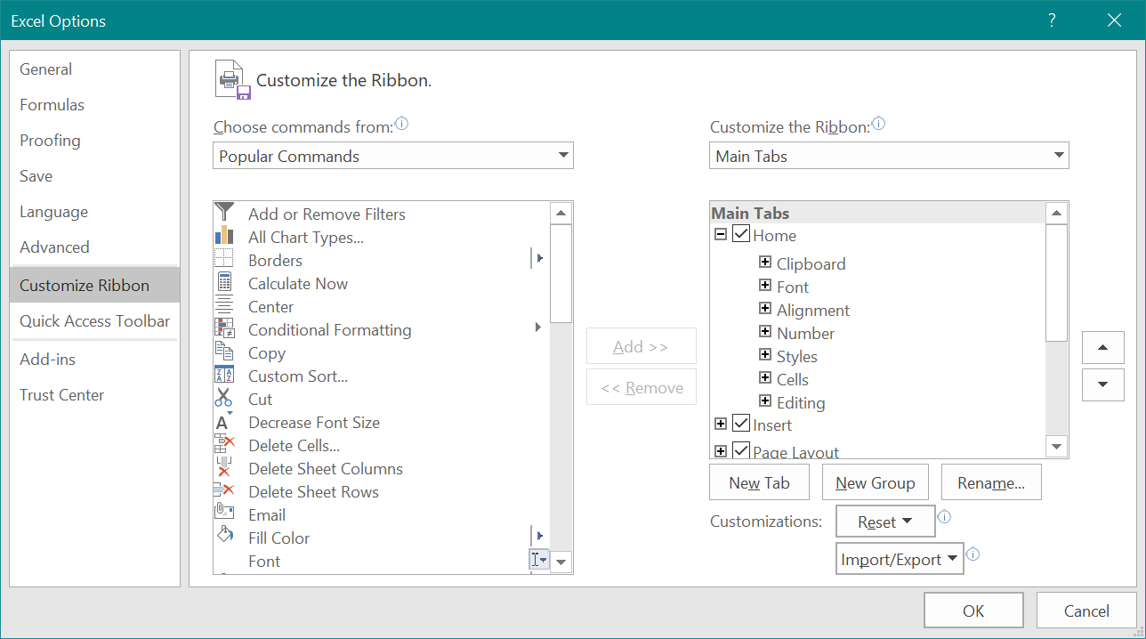
There are two drop-down menus in the right pane, “Choose Commands” and “Customize the Ribbon”. Select the desired items and move to the desired tabs. You can also enable, disable, reorder and regroup the tabs. If something goes wrong, click “Reset All Customizations” in the “Customize” drop-down menu to set the ribbon back to the initial settings.

Related: How to Fix Slow Excel?

Show or Hide the Ribbon in Excel Mac

Similar to Windows, you can also use shortcuts and customize the appearance of the Ribbon in Mac.

1. Use shortcut keys to toggle the Ribbon in Excel Mac

Just press the “Command + Option + R” shortcut keys to toggle the ribbon on Excel. This means the ribbon will be displayed when you press the shortcut keys for the first time, and then hidden when you press them for the second time.

2. Use the arrows to hide or show the ribbon

Another simplest method on a Mac is to click the arrow near the upper right corner. This arrow will appear when the ribbon is visible and will appear when it is hidden. Click it to show or hide the ribbon as needed.

3. Turn off the ribbon from Excel Preferences

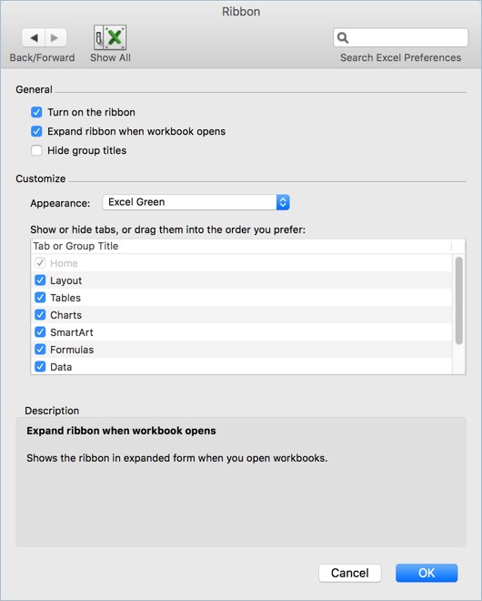
You can permanently turn off the ribbon on Excel to free up some space. Press “Command + ,” keys or go to the “Excel > Preferences…” menu. Click the “Ribbon” option in the Preferences dialog box.

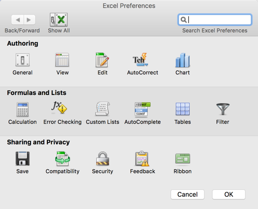
In the Ribbon dialog, uncheck the “Turn on the Ribbon” box. Also remember that the “Command + Option + R” shortcut will work on Mac Excel, provided you have turned on the Ribbon in the preferences.

4. Hide the ribbon when the workbook is opened

Another option is to hide the ribbon when opening a new workbook. To enable this option, go to the Excel Ribbon Preferences and uncheck the “Expand the ribbon when the workbook is opened” option. Once you have a workbook open, you can use the arrows or shortcut keys to toggle the ribbon appearance.

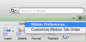
You can also click the gear icon and go directly to the ribbon preferences.

Related: Convert rows to columns and columns to rows in Excel.

5. Click the menu in Excel Office 365

If you’re using Excel on a Mac with an Office 365 subscription, you can switch the ribbon with just a click of a menu item.

Customize the Ribbon in Mac

Similar to Windows Excel, you can also customize the tab order in Mac by selecting the Customize Ribbon Tab Order option from the gear icon. For convenience, you can change the order and rearrange the icon tools.