5 Ways to Calculate Inverse Sine in Microsoft Excel

Are you a math student or working on a data analysis project involving trigonometric functions? Wondering if you can calculate the inverse sine function using Excel? Yes, you can!

In addition to data analysis and visualization, Excel is also a suitable software for solving math and statistics problems. Microsoft Excel comes with more than 50 formulas to solve math and trigonometric problems.

In addition to built-in formulas, you can also create custom functions and procedures to calculate inverse sine in Excel using Excel VBA, Power Query, Office Scripts, etc.

If you need to solve complex problems involving inverse sine or just want to build an inverse sine calculator, you have come to the right place.

Read on to learn more about the inverse sine function, when you might need it, and several intuitive ways to perform the inverse sine function in Excel.

Recommendation: Multi-vendor Marketing Community WordPress Theme REHub

What is the inverse sine function?

The inverse sine function is a mathematical operation that finds the angle whose sine value matches a given number. It is usually expressed as sin^(-1) or inverse sine. In simple language, it is the inverse of the sine function.

For given values ​​-1 and 1, the inverse sine function returns the angle (in radians or degrees) whose sine is equal to that value. Mathematically, if y = sin^(-1)(x), then sin(y) = x.

You may want to notice that the principal values ​​of the inverse sine function are between -π/2 and π/2 radians or -90° and 90° in degrees.

Reasons for Calculating the Inverse Sine Function

Here’s why you might need to calculate the inverse sine:

1. You want to find the angle in degrees or radians whose sine matches a given number.
2. The inverse sine calculation helps you solve physics, engineering, and math problems involving angles and waves.
3. If you are designing and analyzing mechanical systems with rotating parts, there may be times when you need to calculate the inverse sine.
4. This function also helps in understanding oscillatory behavior and periodic phenomena in different disciplines.
5. If you are interested in computer graphics and game development and want to use it to manipulate angles and rotations
6. The inverse sine is also important in navigation and astronomy for celestial calculations and positioning.
7. In signal processing, you often need to calculate the inverse sine when you need to calculate the phase angle to understand a waveform.

So far, you have learned the definition of inverse sine and its applications in mathematics and real life. Now, let’s explore how to calculate inverse sine in Excel.

Use formulas to calculate inverse sine

This Product Code function in Excel formula helps you calculate inverse sine in Excel. If you have a right triangle, the sine of that angle will be the ratio of the lengths of the opposite side and the hypotenuse.

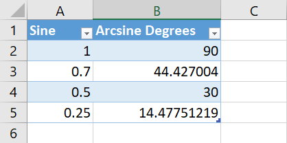
The sine function is a function of -1 and 1 as the angle varies from 0 to 90 degrees (or 0 to π/2) in a right triangle, in radians. Therefore, you can calculate the sine of any given number between 1 and -1. For example, 0.7.

The inverse function of sine, or inverse sine, is the angle between the hypotenuse and the opposite side. If the sine is the given number 0.7, then its inverse sine is 0.775397496610753, in radians.

If you convert this to degrees, which is a more common unit for angles, you get 44.4270040008057° or 44.42°.

Suppose you have a table of values ​​for the height and hypotenuse of a right triangle. You must find the corresponding inverse sine value. Here is how to use the ASIN function in Excel:

Recommendation: WordPress Activity Log Plugin WP Activity Log Pro 

Calculate the arc sine value using ASIN in Excel

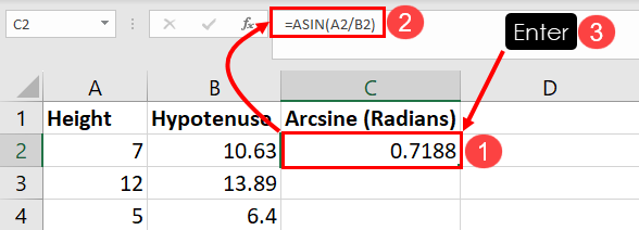
1. Highlight the first cell of the table that needs to be filled with the arc sine value.
2. Double-click and enter the following formula:

=ASIN(A2/B2)

3. Press enter to get the arcsine value in radians.

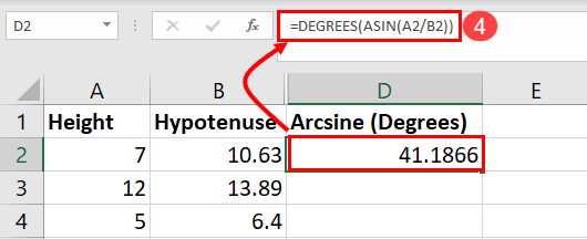
4. If you need to get the inverse sine value in degrees, enter the following formula:

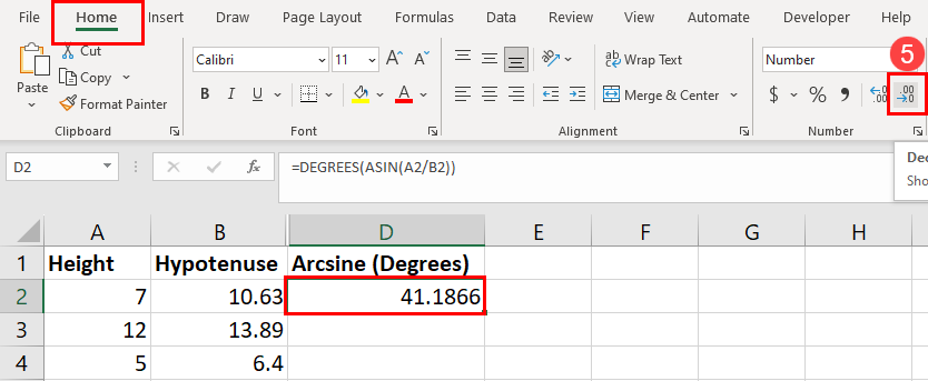
=DEGREES(ASIN(A2/B2))

5. The above formula generates multiple decimal values. Use the Reduce Decimals or Increase Decimals tools on the Home tab on the Excel ribbon menu to reduce or increase decimals.

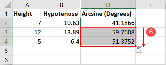
6. After generating the inverse sine value for the first cell in the table, use the fill handle to calculate the inverse sine of its co-sine value.

Need to modify the above formula to make it work in your own worksheet? Please follow the instructions below:

• A2 should be the height of the right triangle
• B2 should be the hypotenuse of the triangle

Suppose you only know the ratio of the opposite side to the hypotenuse of a few right triangles and need to calculate the inverse sine in Excel. Here is how to put the formula in the target cell of the product code:

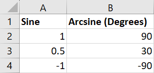
=DEGREES(ASIN(0.5))

In the above formula, 0.5 is the sine number given in the math engineering problem.

Calculate the inverse sine function using Power Query

In Power Query, you can calculate the inverse of sine from a sine number using the Number.ASIN and Number.PI functions. Detailed instructions are as follows:

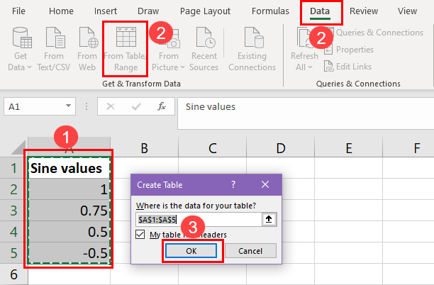
1. Highlight the entire column of sine numbers that need to be converted to arc sine.
2. Click on the Data tab, and then click on the From Table/Range button.
3. Now, click on OK in the Create Table dialog box.

4. Your dataset will be loaded into the Power Query Editor tool.
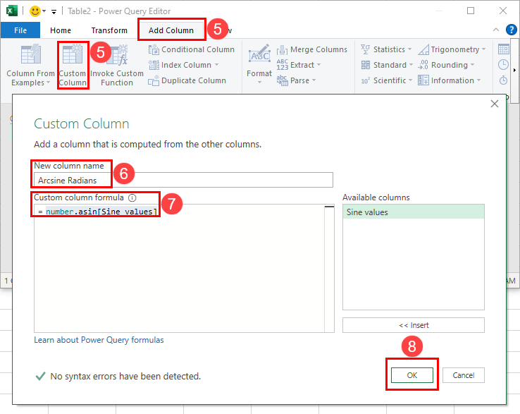
5. There it is. Click the Add Row button, then click Custom Row.
6. In the New Column Name field, type Inverse Sine Radians.
7. In the Custom Column Formula field, type the following formula:

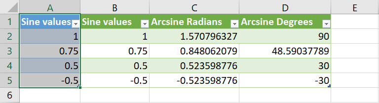
=Number.Asin([Sine values])

8. Click OK to add a new column with the inverse sine values ​​in radians.

9. To convert radian values ​​to degrees, add a custom column again and use the following formula:

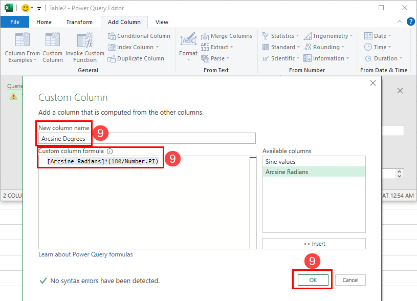
=[Arcsine Radians]*(180/Number.PI)

10. You should now see a column with the arc sine in degrees.

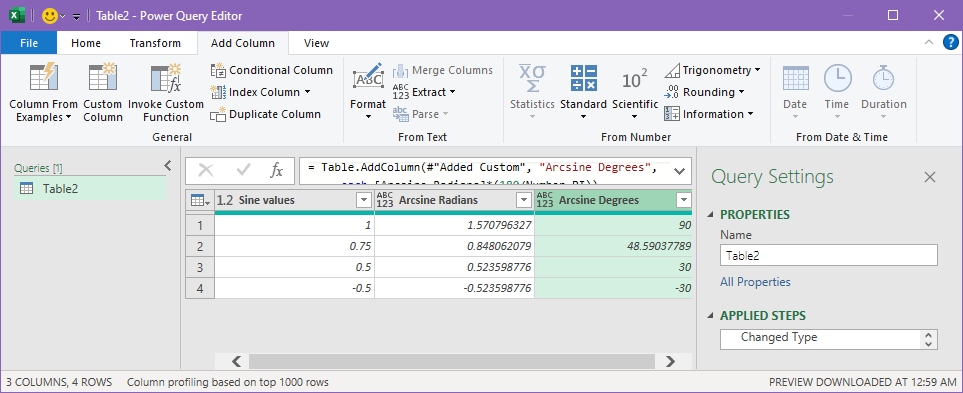
11. Click File and select Close and load to option.

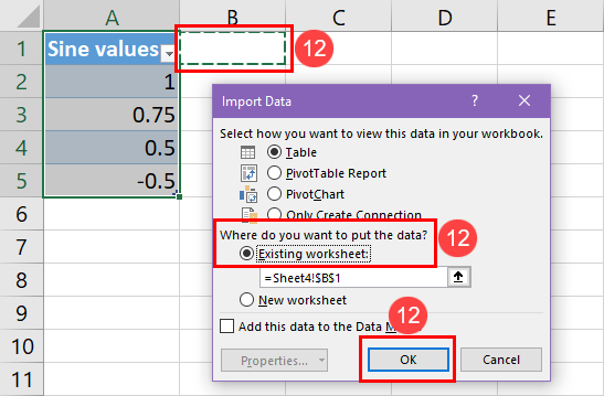
12. In the Import Data dialog box, select Existing worksheet options and select the cells to import the columns into.

How to calculate inverse sine values ​​in Excel using Power Pivot

In Power Pivot, you can use German DAX Index (Data Analysis Expression) language.

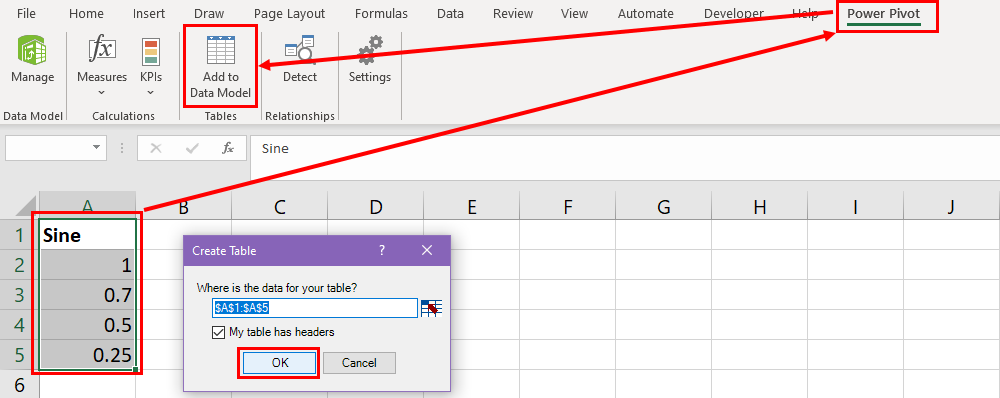
This assumes that you have already imported your data into Power Pivot. If not, you can import your data by going to the Power Pivot menu, clicking the Power Pivot tab, and selecting Add to Data Model.

To add source data columns to Power Pivot, follow these steps:

1. You should now see the Power Pivot window on your workbook.
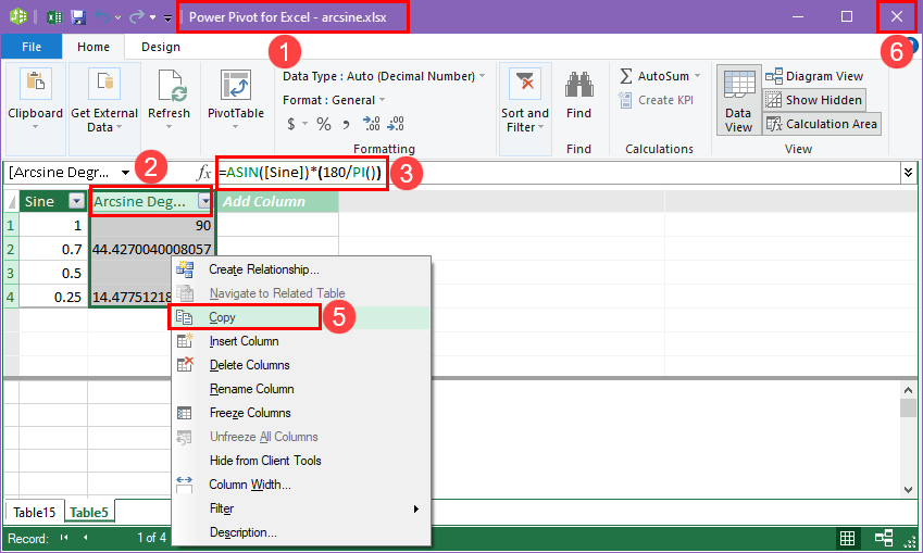
2. Double-click the Add Column text and rename it Inverse Sine.
3. Click the Formula bar and copy and paste the following formula into it:

=ASIN([Sine])*(180/PI())

4. Select the calculated column.
5. Right-click and select Copy.
6. Close the Power Pivot window.

7. Select the cells where you want to paste the columns in Power Pivot.
8. Hit Ctrl + Alt + F and select CSV.

9. Click OK to import the calculated columns into the worksheet.

You can find Power Pivot as a tab in modern Excel desktop applications such as Excel for Microsoft 365, Excel 2021, Excel 2019, and more. In older desktop versions of Excel, you would find this in Developers > Excel Add-ins.

Recommended:  Best WordPress LMS Plugin Masteriyo LMS 

Calculate the Inverse Sine Function in Excel Using Excel VBA

Don’t want to manually calculate the inverse sine of a large data set? Use the following Excel VBA script. In addition, you’ll find easy steps to work with the code:

1. Click the Developer tab on the Excel Ribbon Menu.
2. Select the Visual Basic button to bring up the Excel VBA Editor interface.

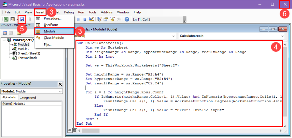
3. Click Insert and select Module.
4. In the new module, copy and paste the following Excel VBA script:

Sub Calculatearcsin() Dim ws As Worksheet Dim heightRange As Range, hypotenuseRange As Range, resultRange As Range Dim i As Long Set ws = ThisWorkbook.Worksheets("Sheet2")
 Set heightRange = ws.Range("A2:A4") Set hypotenuseRange = ws.Range("B2:B4") Set resultRange = ws.Range("C2:C4")
 For i = 1 To heightRange.Rows.Count If IsNumeric(heightRange.Cells(i, 1).Value) And IsNumeric(hypotenuseRange.Cells(i, 1).Value) And hypotenuseRange.Cells(i, 1).Value 0 Then resultRange.Cells(i, 1).Value = WorksheetFunction.Degrees(WorksheetFunction.Asin(heightRange.Cells(i, 1).Value / hypotenuseRange.Cells(i, 1).Value)) Else resultRange.Cells(i, 1).Value = "Error: Invalid input" End If Next i End Sub 

5. Click the Save button.
6. Close the Excel VBA Editor tool.

7. Press Alt + F8 to open the Macro dialog.
8. There, select the Calculate Inverse Sine macro and click Run to execute the VBA script.

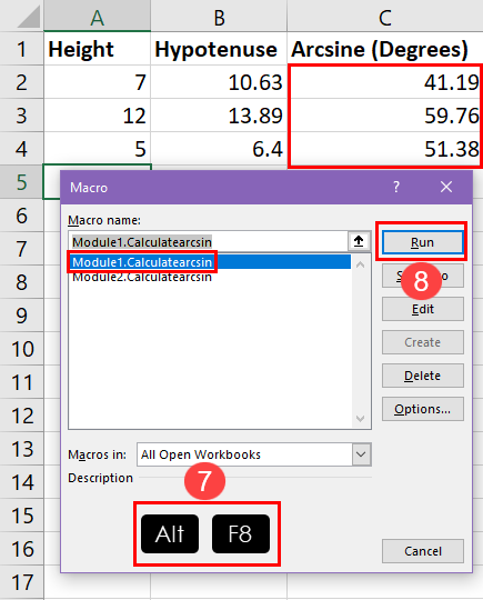
The above code will automatically calculate the inverse sine (in degrees) for the range of cells C2:C4 if you have the height of a few right triangles from A2:A4 and the hypotenuse B2:B4.

If your data set is larger and the values ​​are in a different range of cells than mentioned in this tutorial, you will have to modify the script. Here are the instructions for modifying the script:

• "A2:A4": This cell range should contain the triangle height data, modify it accordingly.
• "B2:B4": Similarly, you should enter the triangle hypotenuse data in this cell range, or modify it according to your own data set.
• "C2:C4": This is the cell range that Excel will fill with the arcsine values. Modify this cell range as well if needed.
• "Sheet2": This is the worksheet where the macro will work. Please change it according to your workbook.

Suppose you have only sine values ​​in your data set and you need to get the corresponding inverse sine value or angle. Here is a VBA script you can use:

Sub CalculateInverseSineInDegrees() Dim ws As Worksheet Dim sineRange As Range, resultRange As Range Dim i As Long
 Set ws = ThisWorkbook.Worksheets("Sheet2") Set sineRange = ws.Range("A2:A10") Set resultRange = ws.Range("B2:B10")
 For i = 1 To sineRange.Rows.Count If IsNumeric(sineRange.Cells(i, 1).value) Then Dim value As Double value = sineRange.Cells(i, 1).value If value >= -1 And value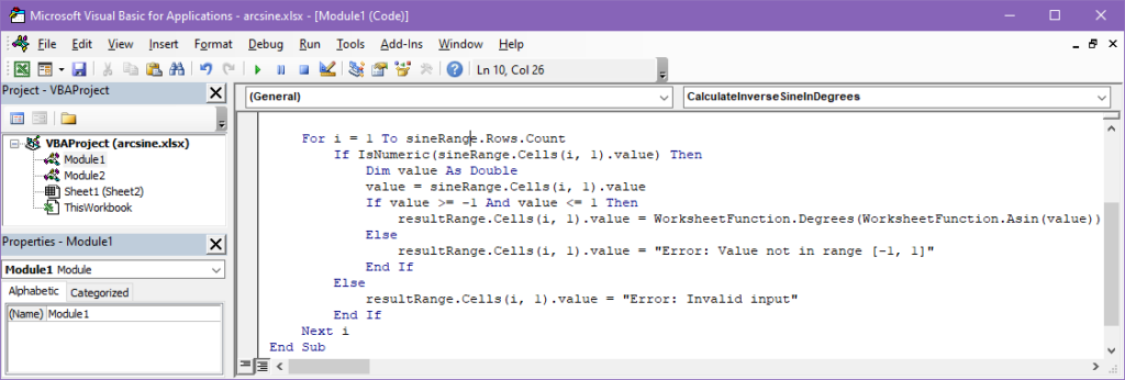 

In the code above, the cell range "A2:A10" has the sine numbers to be converted to arc sine. The arc sine calculator populates the results into "B2:B10". The code calculates the arc sine in Excel in degrees.

Recommendation: WordPress Member Plugin Restrict Content Pro + Addons

Use Office Script to Create an Inverse Sine Calculator

Do you often need to calculate the inverse sine function in the Excel web application by following the manual steps below Product Code function?

Don’t waste time anymore, learn how to use Office Script in Excel. This method also works for Excel in the Microsoft 365 desktop app when connected to the internet. Here are the steps you must follow:

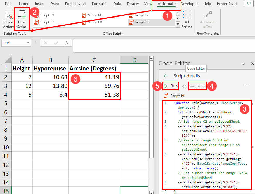
1. Click the Automation tab in the Excel Ribbon.
2. Select the New Script button.
3. Copy and paste the following script in the Code Editor interface:

function main(workbook: ExcelScript.Workbook) {
let selectedSheet = workbook.getActiveWorksheet();
// Set range C2 on selectedSheet
selectedSheet.getRange("C2").setFormulaLocal("=DEGREES(ASIN(A2/B2))");
// Paste to range C3:C4 on selectedSheet from range C2 on selectedSheet
selectedSheet.getRange("C3:C4").copyFrom(selectedSheet.getRange("C2"), ExcelScript.RangeCopyType.all, false, false);
// Set number format for range C2:C4 on selectedSheet
selectedSheet.getRange("C2:C4").setNumberFormatLocal("0.00");
}

4. Click on Save Script option to save your script.
5. Hit Run button to execute the Office Script Code.

If the height and hypotenuse values ​​are obtained in the cells A2:B4, then the above code will fill the cell range C2:C4 with the arc sine values ​​in degrees. The code will also scale the decimal part to two decimal places.

Here’s how to personalize the code to your dataset:

• Change all occurrences of cell C2 to the first cell in your dataset where the inverse sine calculation begins.
• Modify the code element A2/B2 to use the proper syntax for the hypotenuse to represent the height.
• The code copies the formula from C2 to C3:C4. If you performed the same operation in another cell, say D2, then C3:C4 should be D3:D4 or D depending on the length of the D column.

If you only have sine values ​​in your worksheet, use the following Office Scripts code:

function main(workbook: ExcelScript.Workbook) {
let selectedSheet = workbook.getActiveWorksheet();
// Set range B2 on selectedSheet
selectedSheet.getRange("B2").setFormulaLocal("=DEGREES(ASIN(A2))");
// Paste to range B3:B4 on selectedSheet from range B2 on selectedSheet
selectedSheet.getRange("B3:B4").copyFrom(selectedSheet.getRange("B2"), ExcelScript.RangeCopyType.all, false, false);
}

In this script, "B2" is the target cell for the calculation, and A2 is the source cell for the sine value.

Considering that you will be calculating the inverse sine function next to the source data row, "B3:B4" is the range of cells from which the above code will copy and paste the formula B2.

📝 Note: Office Scripts is only available if you have a Microsoft 365 Business Standard subscription or higher. Most Microsoft 365 plans offered by enterprises come with Office Scripts. If you don’t see the Automate tab in Excel for the web or Excel for Microsoft 365 desktop app, you can’t use the feature.

Conclusion

Calculating inverse sine in Excel will be a value-added skill if you are likely to work on Excel projects involving mathematics, trigonometry, engineering, sound waves, etc.

Try the above method with your own data set and you will see how easy it is to implement this skill in real life.

Don’t forget to write about your experience implementing the above method in the comment box below.

Recommendation:  Fix ERR_CONNECTION_TIMED_OUT Error in Chrome